This is the first post of a series on some random(pun intended) topics related to random partial differential equations. Starting with random walk process (i have to start somewhere).

Disclaimer, I am doing this to understand and visualize the random experiments not doing any math. I am literally too old for this.

Starting with wiki blurb:

In mathematics, a random walk, sometimes known as a drunkard’s walk, is a stochastic process that describes a path that consists of a succession of random steps on some mathematical space.

After some reading online, I was confused about the difference between random walk and brownian walk. From SO answer, I found this answer which is interesting way to describe both random walk and Brownian motion(later post)

A Brownian Motion is a continuous time series of random variables whose increments are i.i.d. normally distributed with 0 mean.

A random walk is a discrete process whose increments are +/-1 with equal probability.

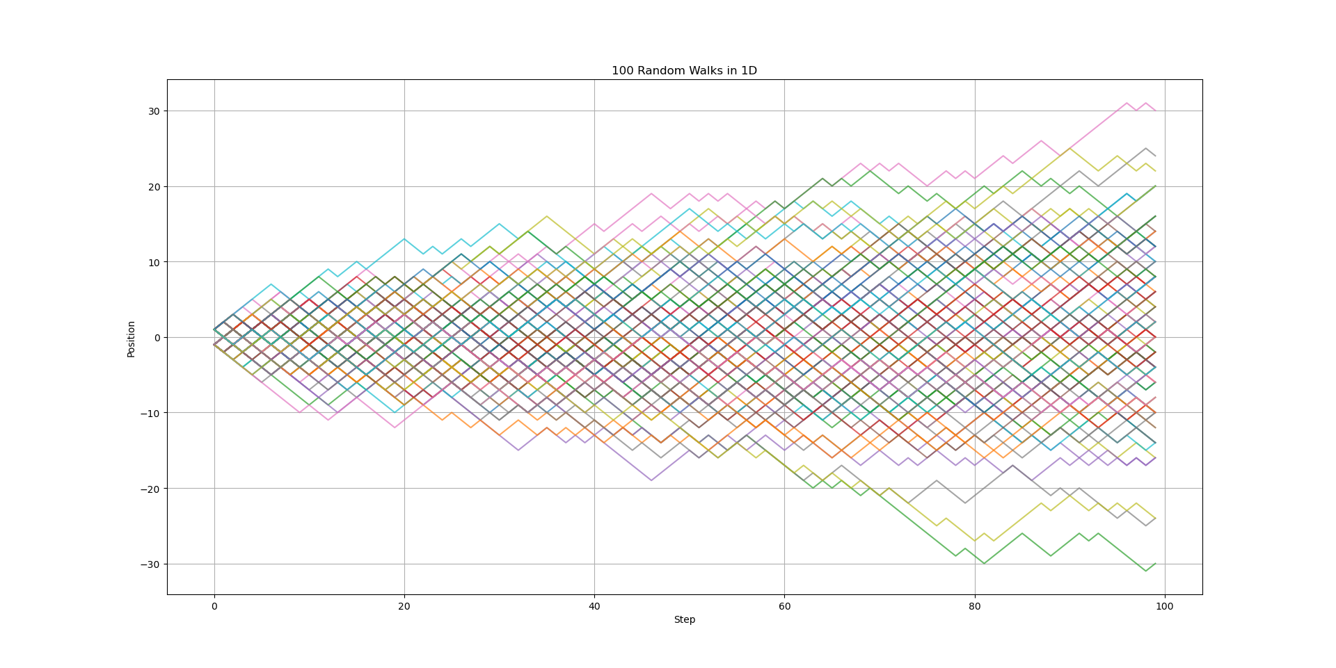
Random Walk 1D Link to heading

The first simulation is 1-D random with [-1:1] with equal probability

import numpy as np
import matplotlib.pyplot as plt

n_steps = 100
n_walks = 100

for _ in range(n_walks):
    steps = np.random.choice([-1, 1], size=n_steps)
    position = np.cumsum(steps)
    plt.plot(position, alpha=0.7)

plt.title(f'{n_walks} Random Walks in 1D')
plt.xlabel('Step')
plt.ylabel('Position')
plt.grid(True)
plt.show()

The pattern is beautiful with large number of walks and steps

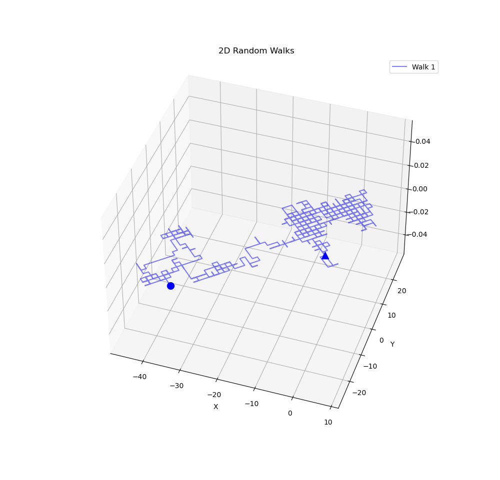
Random Walk 2D Link to heading

To generalize the random walk to 2-D, We can use the following snippet which generate a cool graph

import numpy as np
from mpl_toolkits.mplot3d import Axes3D
import matplotlib.pyplot as plt

def random_walk_2d(steps=1000):
    x_steps = np.random.choice([-1, 1], size=steps)
    y_steps = np.random.choice([-1, 1], size=steps)
    
    x = np.cumsum(x_steps)
    y = np.cumsum(y_steps)
    
    return x, y

# Create 3D plot
fig = plt.figure(figsize=(10, 10))
ax = fig.add_subplot(111, projection='3d')

# Generate multiple random walks
num_walks = 1
steps = 1000
colors = ['b']  # different colors for each walk

for i in range(num_walks):
    x, y = random_walk_2d(steps)
    ax.plot(x, y,  f'{colors[i]}-', alpha=0.5, label=f'Walk {i+1}')
    ax.scatter(x[0], y[0], color=colors[i], s=100, marker='^')
    ax.scatter(x[-1], y[-1],  color=colors[i], s=100, marker='o')

ax.set_xlabel('X')
ax.set_ylabel('Y')
ax.set_title('2D Random Walks')
ax.legend()

plt.show()