Continuing math topics, This is walk through Brownian motion which is good example if stochastic process
Brownian motion is the random motion of particles suspended in a medium (a liquid or a gas).[2] The traditional mathematical formulation of Brownian motion is that of the Wiener process, which is often called Brownian motion, even in mathematical sources.
In mathematics, Brownian motion is described by the Wiener process, a continuous-time stochastic process named in honor of Norbert Wiener.
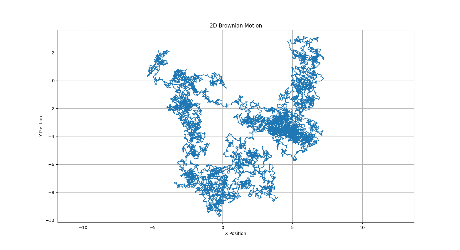
2-D brownian motion Link to heading
Starting with 2-D brownian motion (thanks copilot) with normal distribution to calculate the step and cumsum over x and y.
import numpy as np
import matplotlib.pyplot as plt

def brownian_motion_2d(n_steps, dt=1.0):
    random_steps_x = np.random.normal(0, np.sqrt(dt), size=n_steps)
    random_steps_y = np.random.normal(0, np.sqrt(dt), size=n_steps)

    path_x = np.cumsum(random_steps_x)
    path_y = np.cumsum(random_steps_y)

    return np.concatenate(([0], path_x)), np.concatenate(([0], path_y))

n_steps = 10000
dt = 0.01

x_position, y_position = brownian_motion_2d(n_steps, dt)

plt.figure(figsize=(10, 10))
plt.plot(x_position, y_position)
plt.title('2D Brownian Motion')
plt.xlabel('X Position')
plt.ylabel('Y Position')
plt.grid(True)
plt.axis('equal')
plt.show()
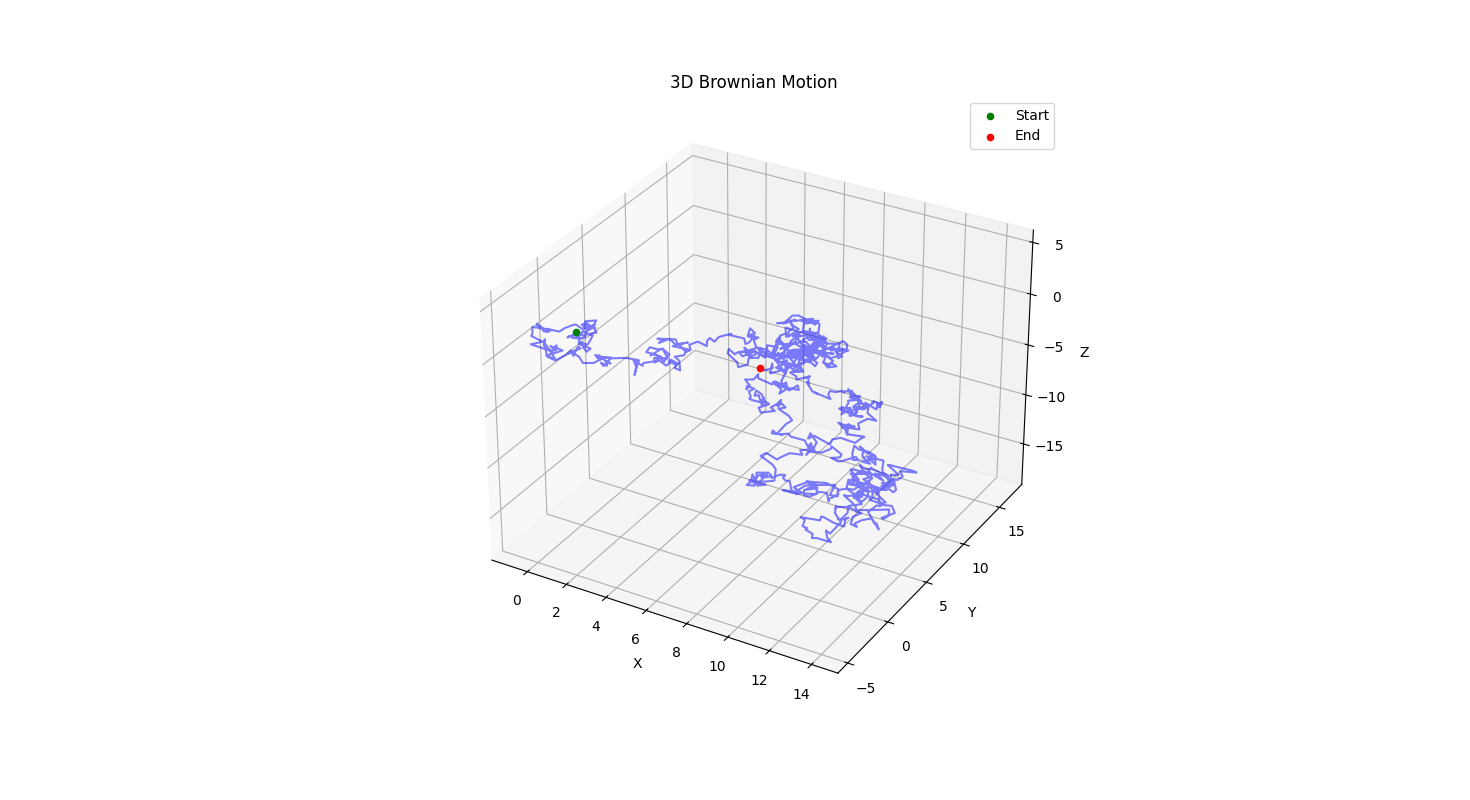
3-D brownian motion Link to heading
To make it more interesting, moving to 3-D with r over the x, y and z.
import numpy as np
from mpl_toolkits.mplot3d import Axes3D

import matplotlib.pyplot as plt

def brownian_motion_3d(n_steps, dt=0.1):
    r = np.random.normal(0, np.sqrt(dt), size=(n_steps, 3))
    positions = np.cumsum(r, axis=0)
    positions = np.vstack([[0, 0, 0], positions])
    return positions

n_steps = 1000

positions = brownian_motion_3d(n_steps)

fig = plt.figure(figsize=(10, 10))
ax = fig.add_subplot(111, projection='3d')
ax.plot(positions[:, 0], positions[:, 1], positions[:, 2], 'b-', alpha=0.5)
ax.scatter(positions[0, 0], positions[0, 1], positions[0, 2], color='green', label='Start')
ax.scatter(positions[-1, 0], positions[-1, 1], positions[-1, 2], color='red', label='End')

ax.set_xlabel('X')
ax.set_ylabel('Y')
ax.set_zlabel('Z')
ax.set_title('3D Brownian Motion')
ax.legend()

plt.show()